Topological phase diagram as a function of spin-orbit coupling

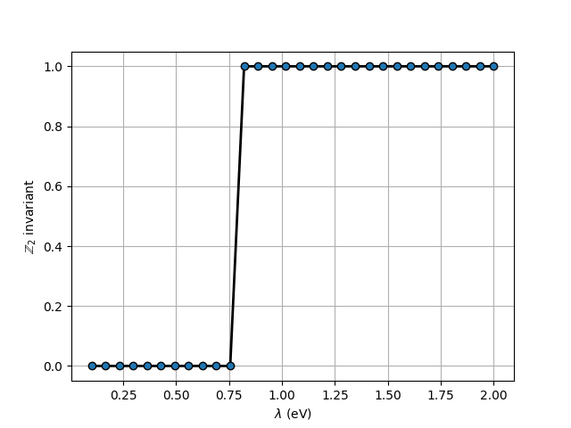
The parameters defined in the configuration file can also be changed after they have been parsed. We use this to update the value of the spin-orbit coupling of the model. By computing the Z2 invariant at different values of the SOC, we can plot the topological phase diagram of a Slater-Koster model.

phase_diagram_bi111.py

from tightbinder.models import SlaterKoster
from tightbinder.fileparse import parse_config_file
from tightbinder.topology import calculate_wannier_centre_flow, calculate_z2_invariant
import matplotlib.pyplot as plt
import numpy as np
from pathlib import Path

def main():
    # Parse configuration file
    path = Path(__file__).parent / ".." / "examples" / "inputs" / "Bi111.yaml"
    config = parse_config_file(path)

    # Init. model
    model = SlaterKoster(config)

    # Generate different values for the spin-orbit coupling and iterate over them
    # At every iteration change SOC value of the model and compute the invariant
    nk = 20
    z2_values = []
    soc_values = np.linspace(0.1, 2, 30)
    for soc in soc_values:

        model.configuration["SOC"][0] = soc
        model.initialize_hamiltonian()

        # Compute and store Z2 invariant
        wcc = calculate_wannier_centre_flow(model, nk, refine_mesh=False)
        z2 = calculate_z2_invariant(wcc)
        z2_values.append(z2)

    # Plot Z2 invariant as a function of SOC
    fig, ax = plt.subplots(1, 1)
    ax.scatter(soc_values, z2_values, marker="o", edgecolors="black", zorder=2.1)
    ax.plot(soc_values, z2_values, "k-", linewidth=2)
    ax.set_ylabel(r"$\mathbb{Z}_2$ invariant")
    ax.set_xlabel(r"$\lambda$ (eV)")
    ax.grid("on")


if __name__ == "__main__":
    main()
    plt.show()

This scripts produces the following diagram: