Density of states

From the band structure one can compute the density of states of the system. To be well-defined, we have to solve the Bloch Hamiltonian not only over a high symmetry path but over the whole Brillouin zone. After meshing the BZ and computing the DoS, we can check that it is properly normalized; we set it so that the integral over all energies is the number of bands:

\[\int \rho(E) dE = N_{bands}\]

density_states.py

from tightbinder.models import SlaterKoster
from tightbinder.fileparse import parse_config_file
from tightbinder.observables import dos
import matplotlib.pyplot as plt
import numpy as np
from pathlib import Path

def main():

    # Parse configuration file and init. model
    path = Path(__file__).parent / ".." / "examples" / "inputs" / "hBN.yaml"
    config = parse_config_file(path)
    model = SlaterKoster(config)

    # Create k point mesh of the Brillouin zone
    nk = 100
    kpoints = model.brillouin_zone_mesh([nk, nk])

    # Solve bands at each kpoint
    model.initialize_hamiltonian()
    results = model.solve(kpoints)

    # Compute density of states
    density, energies = dos(results, delta=0.05, npoints=200)

    # Plot DoS
    fig, ax = plt.subplots(1, 1)
    ax.plot(energies, density, "b-")
    ax.set_ylabel(r"DoS")
    ax.set_xlabel(r"$E$ (eV)")
    ax.grid("on")
    ax.set_xlim([-10, 10])

    # Check normalization
    area = np.trapz(density, energies)
    print(f"Area: {area:.4f}")


if __name__ == "__main__":
    main()
    plt.show()

Which produces the next plot:

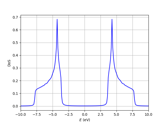
And the following output in terminal: `Area: 1.9993`