Transmission of a nanotube

transport_hydrogen_nanotube

from tightbinder.models import SlaterKoster
from tightbinder.observables import TransportDevice
from tightbinder.fileparse import parse_config_file
import matplotlib.pyplot as plt
from matplotlib.gridspec import GridSpec
import numpy as np
from pathlib import Path

def main():

    # Declare parameters
    length, width = 10, 10

    # Prepare figure for plotting
    fig, ax = plt.subplots(1, 2, figsize=(7, 5))
    ax3d = plt.figure().add_subplot(projection='3d')

    # Parse configuration file
    path = Path(__file__).parent / ".." / "examples" / "inputs" / "chain.yaml"
    config = parse_config_file(path)

    # Init. model
    model = SlaterKoster(config)

    # Generate k points in the 1d system before extending to a nanotube
    nk, labels = 100, ["K", "G", "K"]
    kpoints = model.high_symmetry_path(nk, labels)

    # Append new Bravais vector and extend system along this new directioon (ribbon)
    model.bravais_lattice = np.concatenate((model.bravais_lattice, np.array([[0., 1, 0]])))
    model = model.supercell(n2=width)

    # Compute bands of the ribbon to compare later with the transmission
    # Generate kpoints for the nanotube; nanotube is closed in the width direction (1 cell)
    # while infinite in the length direction.
    model.initialize_hamiltonian()
    results = model.solve(kpoints)

    # Compute Fermi energy to center transmission later
    ef = results.calculate_fermi_energy(model.filling)

    # Plot bands
    labels = ["X", r"$\Gamma$", "X"]
    results.plot_along_path(labels, ax=ax[0])

    # For the transmission, first define the positions of the unit cell of the leads
    # and their periodicity
    left_lead = np.copy(model.motif)
    left_lead[:, :3] -= model.bravais_lattice[0]

    right_lead = np.copy(model.motif)
    right_lead[: , :3] += length * model.bravais_lattice[0]

    period = model.bravais_lattice[0, 0]

    # Finally set a finite ribbon to which we attach the leads
    model = model.reduce(n1=length)

    # Create the transport device and compute the transmission
    model.matrix_type = "sparse"
    device = TransportDevice(model, left_lead, right_lead, period, "default")
    trans, energy = device.transmission(-5, 5, 100)

    # Plot transmission and device
    ax[1].plot(trans, energy - ef, 'k-')
    device.visualize_device(ax=ax3d, pbc=True)
    ax[0].set_ylim([-1.5, 1.5])
    ax[1].set_ylim([-1.5, 1.5])
    ax[1].set_xlabel(r"$T(E)$")


    plt.tight_layout()


if __name__ == "__main__":
    main()
    plt.show()

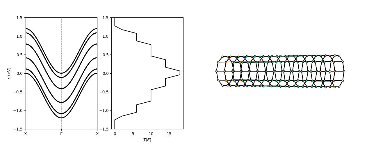
Executing this scripts (which may take some seconds) yields the following plots: