Transmission of a nanoribbon

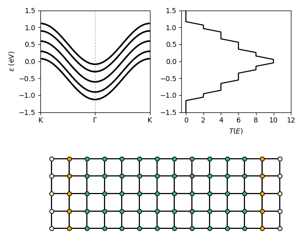
In this example we show how to compute the transmission across a ribbon of hydrogen, and how it compares with the bands as well as the visualization of the device itself.

transport_hydrogen_ribbon.py

from tightbinder.models import SlaterKoster
from tightbinder.observables import TransportDevice
from tightbinder.fileparse import parse_config_file
import matplotlib.pyplot as plt
from matplotlib.gridspec import GridSpec
import numpy as np
from pathlib import Path

def main():

    # Declare parameters
    length, width = 10, 5

    # Prepare figure for plotting
    fig = plt.figure(figsize=(6, 5))
    gs = GridSpec(2, 2, figure=fig)
    ax0 = fig.add_subplot(gs[0, 0])
    ax1 = fig.add_subplot(gs[0, 1])
    ax2 = fig.add_subplot(gs[1, :])
    ax = [ax0, ax1, ax2]

    # Parse configuration file
    path = Path(__file__).parent / ".." / "examples" / "inputs" / "chain.yaml"
    config = parse_config_file(path)

    # Init. model
    model = SlaterKoster(config)

    # Append new Bravais vector and extend system along this new directioon (ribbon)
    model.bravais_lattice = np.concatenate((model.bravais_lattice, np.array([[0., 1, 0]])))
    model = model.reduce(n2=width)

    # Compute bands of the ribbon to compare later with the transmission
    nk, labels = 100, ["K", "G", "K"]
    kpoints = model.high_symmetry_path(nk, labels)
    model.initialize_hamiltonian()
    results = model.solve(kpoints)

    # Compute Fermi energy to center transmission later
    ef = results.calculate_fermi_energy(model.filling)

    # Plot bands
    results.plot_along_path(labels, ax=ax[0])

    # For the transmission, dirst define the positions of the unit cell of the leads
    # and their periodicity
    left_lead = np.copy(model.motif)
    left_lead[:, :3] -= model.bravais_lattice[0]

    right_lead = np.copy(model.motif)
    right_lead[: , :3] += length * model.bravais_lattice[0]

    period = model.bravais_lattice[0, 0]

    # Finally set a finite ribbon to which we attach the leads
    model = model.reduce(n1=length)

    # Create the transport device and compute the transmission
    device = TransportDevice(model, left_lead, right_lead, period, "default")
    trans, energy = device.transmission(-5, 5, 100)

    # Plot transmission and device
    ax[1].plot(trans, energy - ef, 'k-')
    device.visualize_device(ax=ax[2])
    ax[0].set_ylim([-1.5, 1.5])
    ax[1].set_ylim([-1.5, 1.5])
    ax[1].set_xticks([0, 2, 4, 6, 8, 10, 12])
    ax[2].axis("off")
    ax[1].set_xlabel(r"$T(E)$")

    plt.tight_layout()


if __name__ == "__main__":
    main()
    plt.show()

The expected output is: